inst_list = c("tidyverse", "plotly", "png", "ggpubr")

for(i in inst_list){
  if(!inst_list[i] %in% installed.packages()){
    print(inst_list[i])
    install.packages(inst_list[i])
  }
}

library(png)
library(ggpubr)
library(tidyverse)
library(plotly)Workshop Project Report
R
25Winter
data: melb_data.csv
Analysing a dataset in R
We are using the png, ggpubr, tidyverse and plotly libraries to examine our data. We can install and enable these libraries as follows, using an if loop to prevent repeat installation.
Melbourne Housing Data
The dataset we have chosen is the Melbourne Housing Dataset. We can import the data and run a summary as follows:
melb_data_raw <- read.csv("data/melb_data.csv")
summary(melb_data_raw)
X Suburb Address Rooms
Min. : 1 Length:13580 Length:13580 Min. : 1.000
1st Qu.: 3396 Class :character Class :character 1st Qu.: 2.000
Median : 6790 Mode :character Mode :character Median : 3.000
Mean : 6790 Mean : 2.938
3rd Qu.:10185 3rd Qu.: 3.000
Max. :13580 Max. :10.000
Type Price Method SellerG
Length:13580 Min. : 85000 Length:13580 Length:13580
Class :character 1st Qu.: 650000 Class :character Class :character
Mode :character Median : 903000 Mode :character Mode :character
Mean :1075684
3rd Qu.:1330000
Max. :9000000
Date Distance Postcode Bedroom2
Length:13580 Min. : 0.00 Min. :3000 Min. : 0.000
Class :character 1st Qu.: 6.10 1st Qu.:3044 1st Qu.: 2.000
Mode :character Median : 9.20 Median :3084 Median : 3.000
Mean :10.14 Mean :3105 Mean : 2.915
3rd Qu.:13.00 3rd Qu.:3148 3rd Qu.: 3.000
Max. :48.10 Max. :3977 Max. :20.000
Bathroom Car Landsize BuildingArea
Min. :0.000 Min. : 0.00 Min. : 0.0 Min. : 0
1st Qu.:1.000 1st Qu.: 1.00 1st Qu.: 177.0 1st Qu.: 93
Median :1.000 Median : 2.00 Median : 440.0 Median : 126
Mean :1.534 Mean : 1.61 Mean : 558.4 Mean : 152
3rd Qu.:2.000 3rd Qu.: 2.00 3rd Qu.: 651.0 3rd Qu.: 174
Max. :8.000 Max. :10.00 Max. :433014.0 Max. :44515
NA's :62 NA's :6450
YearBuilt CouncilArea Lattitude Longtitude
Min. :1196 Length:13580 Min. :-38.18 Min. :144.4
1st Qu.:1940 Class :character 1st Qu.:-37.86 1st Qu.:144.9
Median :1970 Mode :character Median :-37.80 Median :145.0
Mean :1965 Mean :-37.81 Mean :145.0
3rd Qu.:1999 3rd Qu.:-37.76 3rd Qu.:145.1
Max. :2018 Max. :-37.41 Max. :145.5
NA's :5375
Regionname Propertycount
Length:13580 Min. : 249
Class :character 1st Qu.: 4380
Mode :character Median : 6555
Mean : 7454
3rd Qu.:10331
Max. :21650
Data has been imported to a ‘raw’ data object, to be drawn from to produce usable data.
Data Cleaning
This data includes some values we would like to change before we continue, so we can load the data into a new object for manipulation. From the summary, we can see that the oldest house was built in 1196. Since Melbourne was settled in 1835, this datapoint is a clear outlier and suggests it may be a typo. Therefore we can mutate this datapoint as we load the data into a new object:
melb_data <- melb_data_raw %>% mutate(YearBuilt =
                                        ifelse(YearBuilt < 1800,NA,YearBuilt))
No other clear outliers/typos exist. Landsize of 0 appears to relate to apartments. Postcode, latitude, longitude, distance all within reasonable bounds.
Exploring Data
To explore the data, we can create an object called plot_map to store a ggplot of the data, using the latitude and longitude along the x and y axis. This can then be called with geom_point() to produce a plot.
plot_map <- ggplot(data = melb_data, mapping = aes(x = Longtitude, y = Lattitude))

plot_map + geom_point(mapping = aes(colour = YearBuilt)) +
              theme_classic() + scale_color_viridis_c()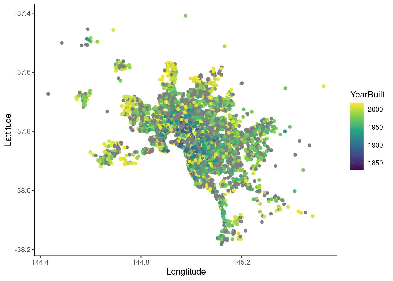
This graph uses the latitude and longitude attributes of the dataset to produce a scatterplot of all house sales in Melbourne, the sum of these data points approximates the geography of Melbourne. The colours can show some hotspots for builds during certain years.
We can overlay this graph on a map of melbourne to show how the areas relate to the real world by taking a map of Melbourne from google and using it as a background image for the graph. This is read in using the png library, and limits are set on the x,y coords of graph to fit image:
map_img <- png::readPNG("./data/map_desaturated.png")

plot_map + background_image(map_img) + geom_point((mapping = aes(colour =
              YearBuilt))) + theme_classic() + scale_color_viridis_c() +
              coord_cartesian(xlim = c(144.4,145.7), ylim = c(-38.2, -37.4))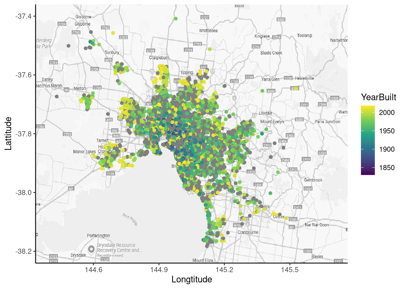
This can alternatively be done using ggmap() rather than an image for the background, however this requires API access.
This data can be aggregated by region as follows:
tooltip_data <- melb_data %>%
  group_by(Regionname) %>%
  summarise(Latitude = median(Lattitude), Longitude = median(Longtitude), Houses =
              sum(Type == "h"), Townhouses = sum(Type == "t"), Units =
              sum(Type == "u"), Properties = n(), Mean_Price = median(Price), PropertySize = median(Landsize))
# A tibble: 8 × 9
Regionname Latitude Longitude Houses Townhouses Units Properties Mean_Price
<chr> <dbl> <dbl> <int> <int> <int> <int> <dbl>
1 Eastern Metr… -37.8 145. 1173 118 180 1471 1010000
2 Eastern Vict… -38.0 145. 50 0 3 53 670000
3 Northern Met… -37.8 145. 2754 307 829 3890 806250
4 Northern Vic… -37.6 145. 41 0 0 41 540000
5 South-Easter… -38.0 145. 388 25 37 450 850000
6 Southern Met… -37.9 145. 2721 425 1549 4695 1250000
7 Western Metr… -37.8 145. 2290 239 419 2948 793000
8 Western Vict… -37.7 145. 32 0 0 32 400000
# ℹ 1 more variable: PropertySize <dbl>This table separates out the median price, latitude, longitude, number of houses/units/townhouses and land size of properties.
The goal was then to use these in plotly to have hoverable aggregated plot points, however I wasn’t able to finish this.
tooltip_map <- ggplot(data = tooltip_data, mapping = aes(x = Longitude, y = Latitude)) + background_image(map_img) + geom_point(data = tooltip_data, label = tooltip_data$Regionname, label2 = tooltip_data$Mean_Price, label3 = tooltip_data$Houses, label4 = tooltip_data$Units) + theme_classic() + scale_color_viridis_c() +
  coord_cartesian(xlim = c(144.4,145.7), ylim = c(-38.2, -37.4))
Warning in geom_point(data = tooltip_data, label = tooltip_data$Regionname, :
Ignoring unknown parameters: `label`, `label2`, `label3`, and `label4`tooltip_map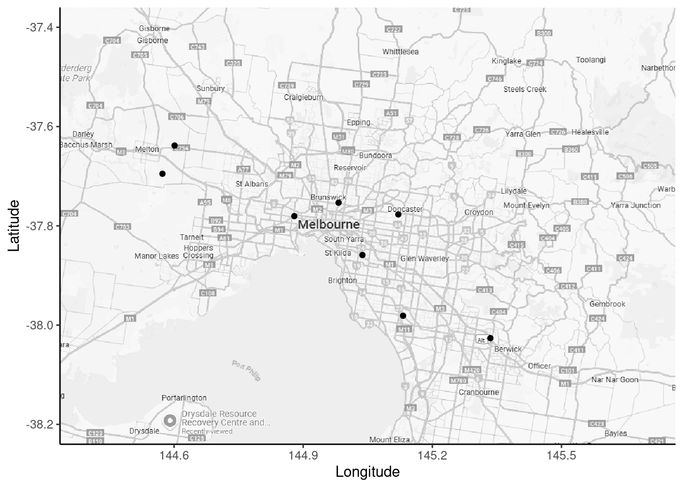
ggplotly(tooltip_map)melb <- read.csv("data/melb_data.csv")
melb |>
summary() |>
knitr::kable()| X | Suburb | Address | Rooms | Type | Price | Method | SellerG | Date | Distance | Postcode | Bedroom2 | Bathroom | Car | Landsize | BuildingArea | YearBuilt | CouncilArea | Lattitude | Longtitude | Regionname | Propertycount | |
|---|---|---|---|---|---|---|---|---|---|---|---|---|---|---|---|---|---|---|---|---|---|---|
| Min. : 1 | Length:13580 | Length:13580 | Min. : 1.000 | Length:13580 | Min. : 85000 | Length:13580 | Length:13580 | Length:13580 | Min. : 0.00 | Min. :3000 | Min. : 0.000 | Min. :0.000 | Min. : 0.00 | Min. : 0.0 | Min. : 0 | Min. :1196 | Length:13580 | Min. :-38.18 | Min. :144.4 | Length:13580 | Min. : 249 | |
| 1st Qu.: 3396 | Class :character | Class :character | 1st Qu.: 2.000 | Class :character | 1st Qu.: 650000 | Class :character | Class :character | Class :character | 1st Qu.: 6.10 | 1st Qu.:3044 | 1st Qu.: 2.000 | 1st Qu.:1.000 | 1st Qu.: 1.00 | 1st Qu.: 177.0 | 1st Qu.: 93 | 1st Qu.:1940 | Class :character | 1st Qu.:-37.86 | 1st Qu.:144.9 | Class :character | 1st Qu.: 4380 | |
| Median : 6790 | Mode :character | Mode :character | Median : 3.000 | Mode :character | Median : 903000 | Mode :character | Mode :character | Mode :character | Median : 9.20 | Median :3084 | Median : 3.000 | Median :1.000 | Median : 2.00 | Median : 440.0 | Median : 126 | Median :1970 | Mode :character | Median :-37.80 | Median :145.0 | Mode :character | Median : 6555 | |
| Mean : 6790 | NA | NA | Mean : 2.938 | NA | Mean :1075684 | NA | NA | NA | Mean :10.14 | Mean :3105 | Mean : 2.915 | Mean :1.534 | Mean : 1.61 | Mean : 558.4 | Mean : 152 | Mean :1965 | NA | Mean :-37.81 | Mean :145.0 | NA | Mean : 7454 | |
| 3rd Qu.:10185 | NA | NA | 3rd Qu.: 3.000 | NA | 3rd Qu.:1330000 | NA | NA | NA | 3rd Qu.:13.00 | 3rd Qu.:3148 | 3rd Qu.: 3.000 | 3rd Qu.:2.000 | 3rd Qu.: 2.00 | 3rd Qu.: 651.0 | 3rd Qu.: 174 | 3rd Qu.:1999 | NA | 3rd Qu.:-37.76 | 3rd Qu.:145.1 | NA | 3rd Qu.:10331 | |
| Max. :13580 | NA | NA | Max. :10.000 | NA | Max. :9000000 | NA | NA | NA | Max. :48.10 | Max. :3977 | Max. :20.000 | Max. :8.000 | Max. :10.00 | Max. :433014.0 | Max. :44515 | Max. :2018 | NA | Max. :-37.41 | Max. :145.5 | NA | Max. :21650 | |
| NA | NA | NA | NA | NA | NA | NA | NA | NA | NA | NA | NA | NA | NA’s :62 | NA | NA’s :6450 | NA’s :5375 | NA | NA | NA | NA | NA |